Simple Linear Regression

Regression is a statistical tool for investigating the relationships between variables. Simple linear regression is the simplest form of regression; it creates a linear model for the relationship between the dependent variable and a single independent variable. Visually, simple linear regression "draws" a trend line on the scatter plot of two variables that best approximates their linear relationship. The model can be expressed with the two parameters of its line: slope and intercept. Other models use more parameters for more complex curves. This is one of the most popular tools in statistics, and it is frequently used as a predictor for machine learning.

Explanation and history

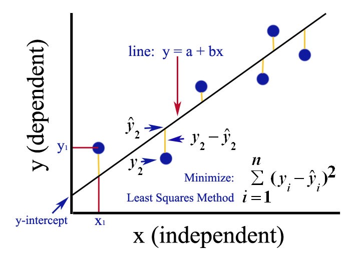
At the core of linear regression is the method of least squares. In this method, the linear trend line is chosen which minimizes the sum of every data point’s squared residual (deviation from the model).

The method of least squares was independently discovered by Carl Friedrich-Gauss and Adrien-Marie Legendre in the early 19th century. The linear regression methods used today can be primarily attributed to the work of R.A. Fisher in the 1920s.

Use-cases

In simple linear regression, both the independent and dependent variables must be numeric. The dependent variable (y) can then be expressed in terms of the independent variable (x) using the two line parameters intercept (a) and slope (b) with the equation y = a + b * x. For these approximations to be meaningful, the dependent variable should take continuous values. The relationship between any two variables satisfying these conditions can be analyzed with simple linear regression. However, the model will only be successful for linearly related data. Some common examples include:

Predicting housing prices with square footage, number of bedrooms, number of bathrooms, etc.
Analyzing sales of a product using pricing or performance information
Calculating causal relationships between parameters in biological systems

Constraints

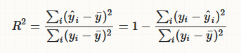
Because simple linear regression is so straightforward, it can be used with any numeric data pair. The real question is how well the best model fits the data. There are several measurements which attempt to quantify the success of the model. For example, the coefficient of determination (r²) is the proportion of the variance in the dependent variable that is predictable from the independent variable. A coefficient r² = 1 indicates that the variance in the dependent variable is entirely predictable from the independent variable (and thus the model is perfect).

Example

Let’s look at a straightforward example—predicting short term rental listing prices using the listing’s number of bedrooms. Run :play http://guides.neo4j.com/listings and follow the import statements to load Will Lyon’s rental listing graph.

First initialize the model

CALL regression.linear.create('airbnb prices')

Then add data point by point

MATCH (list:Listing)-[n:IN_NEIGHBORHOOD]->(hood:Neighborhood {neighborhood_id:'78704'})
WHERE exists(list.bedrooms)
    AND exists(list.price)
    AND NOT list:Trained
CALL regression.linear.add('airbnb prices', [list.bedrooms], list.price)
SET list:Trained
RETURN *

Next predict price for a four-bedroom listing

RETURN regression.linear.predict('airbnb prices', [4])

Or make and store many predictions

MATCH (list:Listing)-[:IN_NEIGHBORHOOD]->(:Neighborhood {neighborhood_id:'78704'})
WHERE exists(list.bedrooms) AND NOT exists(list.price)
SET list.predicted_price = regression.linear.predict('airbnb prices', [list.bedrooms])

You can remove data

MATCH (list:Listing {listing_id:'2467149'})-[:IN_NEIGHBORHOOD]->(:Neighborhood {neighborhood_id:'78704'})
CALL regression.linear.remove('airbnb prices', [list.bedrooms], list.price)
REMOVE list:Trained

Add some data from a nearby neighborhood

MATCH (list:Listing)-[:IN_NEIGHBORHOOD]->(:Neighborhood {neighborhood_id:'78701'})
WHERE exists(list.bedrooms)
    AND exists(list.price)
    AND NOT list:Trained
CALL regression.linear.add('airbnb prices', [list.bedrooms], list.price)
SET list:Trained RETURN list

Check out the number of data points in your model

CALL regression.linear.info('airbnb prices')
YIELD model, framework, hasConstant, numVars, state, N, info

Make sure that before shutting down the database, you store the model in the graph or externally

MERGE (m:ModelNode {model: 'airbnb prices'})
SET m.data = regression.linear.data('airbnb prices')

Delete the model

CALL regression.linear.delete('airbnb prices')
YIELD model, framework, hasConstant, numVars, state, N, info

And then when you restart the database, load the model from the graph back into the procedure

MATCH (m:ModelNode {model: 'airbnb prices'})
CALL regression.linear.load('airbnb prices', m.data)
YIELD model, framework, hasConstant, numVars, state, N, info
RETURN model, framework, hasConstant, numVars, state, N, info

Now the model is ready for further data changes and predictions!

Syntax

The simple linear regression procedures were created so that the same procedures may be used for multiple linear regression. Therefore, independent variable must be specified [in brackets] and you must specify number of variables (1) at time of creation as well as the type of model you would like to create ("Simple").